Experiment 0 Measurement and Graphical Analysis
The aim of a typical scientific study or experiment is to investigate how a particular physical quantity is related to another. In such an experiment, the value of the first quantity (the independent variable) is varied, and the value of the second quantity (the dependent variable) is measured. The result is two sets of values corresponding to the two quantities. For example, assume that you performed an experiment that involved monitoring the growth of a fast-growing indoor plant, in a sunny location in your house. In the experiment, you measured the plant's height every 12 hours and recorded the results as shown in Table 0.3. Since a regular ruler was used for measurements, you estimated the error in the plant’s height to be about 1 mm.
| Elapsed Time $x\,\text{(day)}$ | Plant's Height $y \; \pm 0.1\,\text{(cm)}$ |
| $0.5$ | $39.6$ |
| $1.0$ | $39.9$ |
| $1.5$ | $40.3$ |
| $2.0$ | $40.7$ |
| $2.5$ | $40.9$ |
| $3.0$ | $41.3$ |
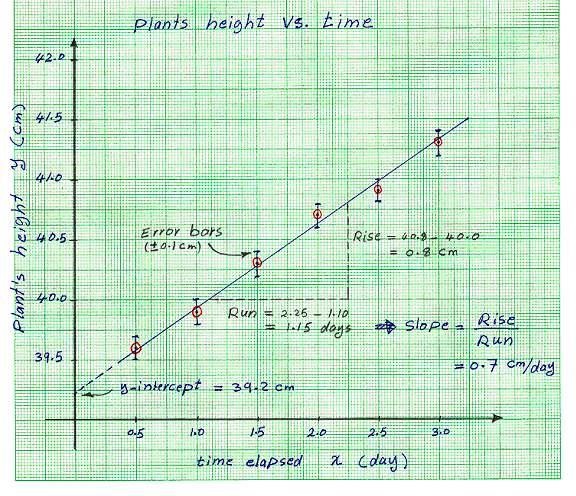
Usually, it is convenient to display tabulated data graphically. The independent variable normally (but not necessarily) is plotted on the horizontal axis while the vertical axis is reserved for the dependent variable. In Figure 0.1, the circled points represent the $x$ and $y$ values in Table 0.3. The vertical bar on each data point shows the range of uncertainty in the corresponding measurement. You probably noticed that the data points on the graph nearly lie on a straight line. This indicates that the linear function $y = m x + b$ is likely to represent the data very well. The best straight line through the data points is called the best linear fit to the data. The parameter $m$ in this equation refers to the slope of the line, and it represents the rate at which $y$ increases with $x$. The other parameter $b$ refers to the $y$-intercept, which represents the initial value of $y$ at $x = 0$.
To find the slope of the linear graph, we need first to mark two points on the straight line and write down their $x$ and $y$ coordinates. Note that these coordinates should be read directly from the linear graph, not from the data table. If the first point has the coordinates $(x_1, y_1)$ and the second point has the coordinates $(x_2, y_2)$, we can calculate the change in $y$ (rise $= \Delta y = y_2 - y_1$) caused by the change in $x$ (run $= \Delta x = x_2 - x_1$). The slope is then calculated as the ratio rise-over-run such that \begin{equation} m = \frac{\text{rise}}{\text{run}} = \frac{y_2 - y_1}{x_2 - x_1} \end{equation} In Figure 0.1, the slope is calculated to be $m = 0.7 \; \text{cm/day}$, which is a relatively high growth rate.
The $y$-intercept ($b$) corresponds to the point at which the linear graph intersects the $y$-axis (at $x = 0$). In Figure 0.1, $b = 39.2 \;\text{cm}$ represents the height of the plant $12$ hours before you took the first measurement. The best linear fit to the data in Table 0.3 is then given by the equation \begin{equation} y = 0.7 \; x + 39.2 \end{equation}