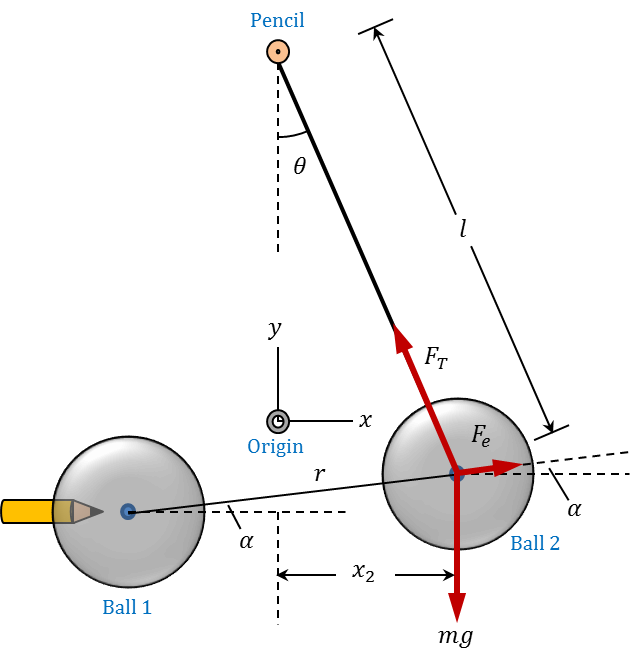
Figure 1.2 shows a schematic diagram of the two charged balls when they are at a distance $r$ from each other. The centre of Ball 1 is located at the coordinates ($x_1, y_1$), while the centre of Ball 2 is at ($x_2, y_2$). Note that the hanging ball experiences three forces: the weight ($mg$), the tension in the string ($F_T$), and the repulsive electrostatic force ($F_e$). Since the system is in static equilibrium, the vector sum of the three forces must be equal to zero.
To determine the electric force and distance between the two balls, you will need the coordinates of their centres while in static equilibrium. In other words, if you know values of $x_1$, $y_1$, $x_2$, and $y_2$, you can substitute in the equations above to calculate $F_e$ and $r$.
The positions of the two balls in different equilibrium states can be obtained by analyzing the different pictures you took in this experiment. The known diameter of the styrofoam balls can be used to scale all position and distance measurements in each picture (see Video 1.1). For this purpose, you are encouraged to use the Logger Pro software, which can be downloaded from here. Note that instructions in this manual are based on version 3.8.6 of the software.
After analyzing all relevant pictures, you will have a set of data that corresponds to the values of $x_1$, $y_1$, $x_2$, and $y_2$ at different equilibrium states of the system. Open a new Logger Pro file and enter these data in four properly labeled columns (see Video 1.2). The next step is to create new columns corresponding to $r$, $\theta$, $\alpha$, and $F_e/mg$, as shown in the table below. For example, to calculate $r$, click on Data in the menu bar and select New Calculated Column from the scroll down menu. Use r for both the name and the short name. For the equation, write sqrt(("x2"-"x1")^2+("y2"-"y1")^2) which corresponds to Equation \ref{lab1_r}. The quotation marks here indicate that you are referring to the entire column of data.
After calculating the new columns, generate a graph of $F_e/mg$ versus $r$. To do that, click in the region to the left of the vertical axis and select Fe/mg then click in the region below the horizontal axis and select r. Adjust the scaling and other axes options by double-clicking anywhere in the graph window. Drag the mouse in the graph window to highlight all data points. Click on Analyze in the menu bar and select Curve Fit from the scroll down menu. Select the Inverse Square general equation and click Try Fit. A curve will be generated, representing the equation F/mg = A/r^2. Save this graph and include it in your lab report.
| $x_1$ ($\text{m}$) |
$y_1$ ($\text{m}$) |
$x_2$ ($\text{m}$) |
$y_2$ ($\text{m}$) |
$r$ ($\text{m}$) |
$\theta$ ($\text{rad}$) |
$\alpha$ ($\text{rad}$) |
$F_e/mg$ |
Do your data support the predictions of Coulomb's law regarding the relation between electric force and distance between two charged objects? Provide a detailed discussion (about 400 words) in this regard. In your discussion, be sure to indicate the limitations of your experiment and the possible sources of error.
Complete the lab report, including all nine sections, as described in the introduction. Submit your lab report by uploading it to the appropriate drop-box.